Simulating a time-varying inductor in Spice
The relationship between the voltage $v_L$ over and the current $i_L$ through an inductor is determined by its inductance $L$:
$$ v_L(t)=L\frac{di_L(t)}{dt}$$
However, this current-voltage relationship is not valid when the inductor is varying in time. For a time variant inductor, the equation modifies to:
$$ v_L(t)=\frac{d}{dt}[L(t).i_L(t)]=L(t)\frac{di_L(t)}{dt}+i_L(t)\frac{dL(t)}{dt}$$
Rearranging this equation gives an expression for the current through the inductor:
$$ i_L(t)=\frac{1}{L(t)}[L(0)i_L(0)+\int_0^t v_L(t) dt] $$
valid if $L(t)\neq 0$ at any time.
We will use this expression to simulate a time-varying inductance in LT Spice. Notice the limitation that $L(t)\neq 0$ at any time.
Suppose we want we simulate a sinusoidal value in function of time with a certain offset: $L(t)$= 5 mH + 3 mH.sin(2π.100 kHz.t). In order to realize this, we have to introduce a custom component in SPICE with the following subcircuit:
.subckt inductor + - params: IL0=0
.func L(time) {5m+3m*sin(2*pi*100k*time)}
gcurr + - value={(sdt(V(+,-))+IL0*L(0))/L(time)}
.ends
The current through the inductor (see equation above) is modeled via a G-type current source gcurr. The integral is realized via the sdt function in SPICE. The initial value at time t=0 of the inductor must be given as parameter.
First, we save the code for this subcircuit into a .txt-file and, for example, place this file in the same folder as your SPICE circuit file.
Next, open the text file in LT Spice, right click on the first word “.subckt”, and select “Create symbol”.
The program asks you if you wish to automatically create a symbol. Click “yes”. A .asy file is created which contains your custom time-varying inductor, typically in the folder 'C:Users\YourUserName\AppData\Local\LTspice\lib\sym\AutoGenerated'
To use the time-varying inductor in a circuit, click “component” (F2) and insert the custom inductor by searching “inductor” in the window.
Plotting the value of the inductance in SPICE in function of time is not straightforward. Let us just check some individual times: we compare the value of the current through and voltage over the inductor (i) in the case of the time-varying inductor at time $t_i$ (after the transition period), and (ii) in the case of a static inductor with value $L(t_i)$.
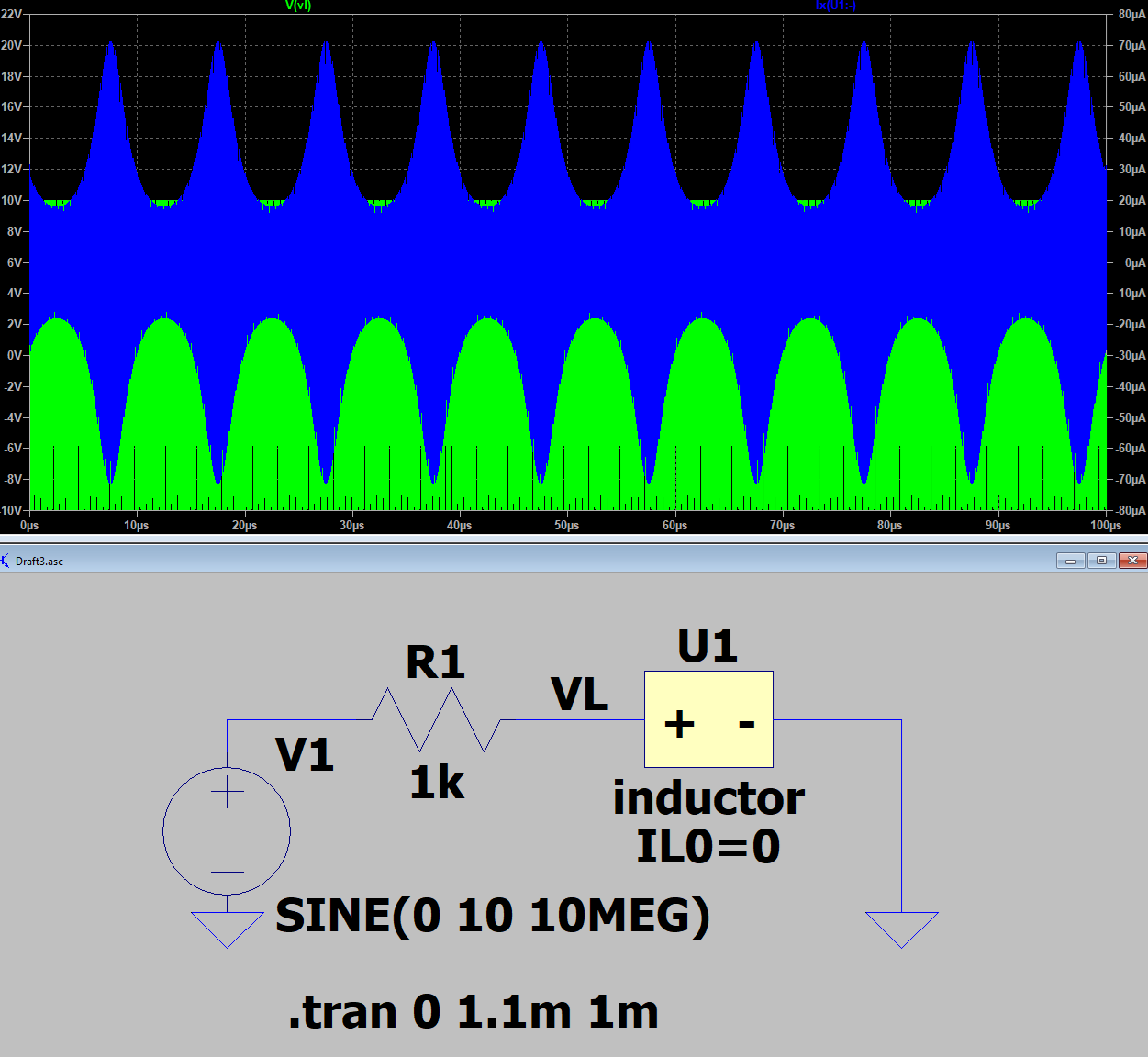
Case (i): We apply a high frequency source in order to create an envelope facilitating comparison between both cases.
At a certain time, e.g., t=50µs, the value of the inductor equals $L$(50µs)= 5 mH + 3 mH.sin(2π.100 kHz.50 µs)=5 mH. If we then zoom in at the simulation at t=50µs, we find the peak value of voltage over and current through the inductor.
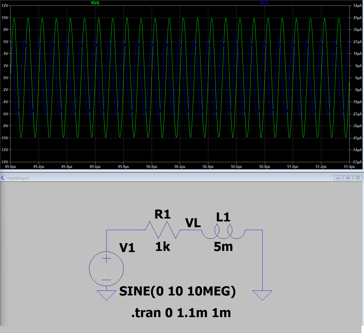
Case (ii): We compare this value with a static inductor of 5 mH:
We find that both the current and voltage correspond to case (i).
We do the same for a lot of other values of time, and always find a correspondence between both cases. This is not a rigid proof, but it gives us sufficient confidence that the inductor was modeled correctly in SPICE.
References
- Biolek, D., Kolka, Z., & Biolkova, V. (2007). Modeling time-varying storage components in PSpice. In Proc. Electronic Devices and Systems IMAPS CS International Conference EDS (Vol. 2007, pp. 39-44).


